This is a surprisingly common problem. Just double-click on one of the tabs (File, Home, Insert, etc.) to make the ribbon reappear (or make it disappear again).

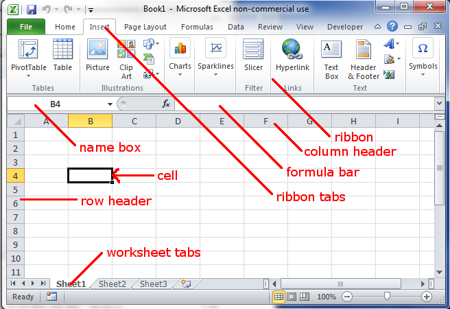
The image above shows some of the basic Excel terminology. Note that the active cell is outlined in bold and has a "handle" (small black square) for dragging in the lower right corner. The name box contains the active cell reference. The formula bar contains the contents of the active cell. The column and row header(s) for the active cell are highlighted.

The image shows one worksheet. The worksheet tabs at the bottom left of the worksheet can be clicked to switch to a different worksheet. The entire document with all the worksheets is called a workbook.

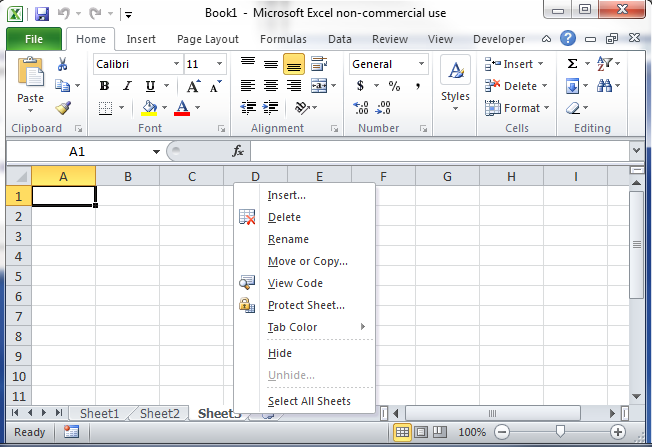
You can right click on a worksheet tab to get the context menu shown in the image above. From there you can rename, delete, copy, move, and insert a worksheet. You can also insert a new worksheet at the end of the workbook by clicking on the rightmost worksheet tab.

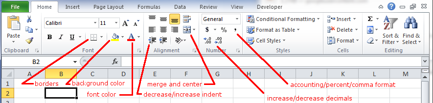
Select the cells you want to format. In the image above, the B2 cell is ready to format. Click on the Home tab of the ribbon. The icons on the ribbon allow quick access to all of the most common formatting options. For more options, click on one of the arrows in the lower right corner of one of the formatting groups.

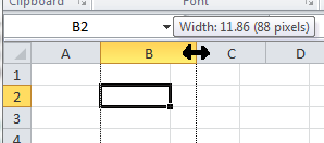
To change the width of a cell you can place the cursor in the column header on the right edge of the column you want to adjust. When the cursor changes to the double arrow, click and drag to the width you want. You can also double click to have Excel automatically change the width to fit the data in the column. You can change the row height by doing the same thing in the row header.

The icons for these quick formats are on the Home tab of the ribbon. The accounting format icon has a $ sign on it. The percent and comma formatting icons have a percent sign and a comma sign on them.

Select all the cells you want to merge together and then click on the Home tab of the ribbon. Then click on . Click on the arrow to the right of it for other merge options such as unmerging cells.

That's easy. Just type the text or number and then move to a different cell by pressing enter, clicking on a different cell, or using the arrow keys.

Just hold down the Alt key while you press the Enter key and Excel will go to a new line at that point. You usually have to modify the row height to see all the text properly.

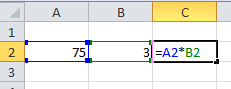
You can enter a formula by entering an = sign and then the formula. Simple formulas consist of cell references and arithmetic operators. The example in the image shows how cell C2 can be set equal to A2 multiplied by B2. Once you press Enter, cell C2 will become 225. You can still see the formula in cell C2 by selecting cell C2 and looking in the formula bar. It is important to use cell references in the formulas instead of the actual numbers so that the C2 cell automatically changes to the right value when cell A2 or cell B2 change.

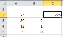
Select the cell with the formula you want to copy. Then click and drag on the black square in the lower right corner of that cell to highlight the whole area you want the formula copied to.

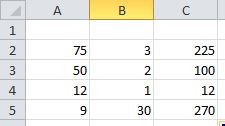
The second image shows the result of copying the formula from C2 into cells C3 through C5. Notice how the formula is automatically adjusted by Excel as it is copied so it is always the product of the cells of the first two columns of the row.

Absolute addressing is used for formulas you want to be able to copy where one of the cells in the formula is in a fixed location.

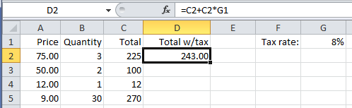
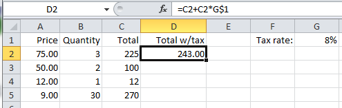
The image above shows regular relative addressing used in a formula. You can see the formula used in cell D2 displayed in the formula bar. The formula works for cell D2.

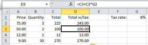
The image above shows what happens when the formula in cell D2 is copied into cells D3 through D5. The formula doesn't work for cells D3 through D5 because Excel increased the row number on all cell references when it copied the formula to lower rows. That was fine for the column C references, but not for the tax rate cell reference (G1). The cell G1 reference has to stay the same. Notice in the formula bar that the reference for G1 has changed to cell G2, which has no value.

The image above shows a modified formula in cell D2. Notice the formula in the formula bar. The reference to cell G1 has been made absolute for the row by placing a $ sign in front of the row number. The dollar sign in front of the row number will keep the row number the same no matter where you copy it to. Many people will also make the column reference absolute in this case ($G$1), but it is not needed unless you plan on copying the formula to other columns.

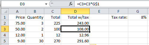
The image above shows the result of copying the formula with the absolute reference. Notice that the formula now works for all the cells in column D. You can see in the formula bar that the formula copied into cell D3 kept the reference to cell G$1 the same.

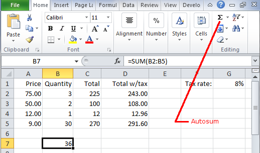
The image above shows how cell values can be summed together using Excel's built-in SUM function. Enter the following to add up the values in cells B2 through B5: =SUM(B2:B5)

You could also have selected all the cells from B2 through B7 and then clicked on the Autosum icon to have Excel enter the formula for you. The Autosum button also has a drop-down list which gives access to other Excel built-in functions.

Specifying a range is easy. Enter the cell reference for the upper-left cell in the range and then enter a colon and the cell reference for the lower-right cell in the range. For example, to sum up all the cells from E3 through E27, enter: =SUM(E3:E27)

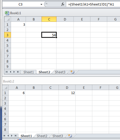
This explanation is going to take advantage of the Excel feature that allows you to click on a cell rather than having to type in its cell reference. Given the image above, how would the formula in cell C2 on worksheet Sheet2 be entered? We want to add cells A1 and D1 on Sheet1 and then multiply that sum by the value in cell A1 on Sheet2.

Do the following:

1. Click on cell C3 on Sheet2
2. Enter: =
3. Enter: (
4. Click on the Sheet1 tab, and then click on cell A1
5. Enter: +
6. Click on cell D1
7. Enter: )
8. Enter: *
9. Click on the Sheet2 tab, and then click on cell A1
10. Enter: Enter

Notice how once you start entering the formula, you keep on entering the formula and don't switch worksheets until you absolutely have to for selecting a cell.

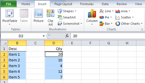
To create a chart, select the cells that you want the chart to reflect. This is easy if the cells are contiguous. If they are not all next to each other, then select the first set of cells that are contiguous, and then hold down the control key as you select the rest of the cells. That was the technique used for the image above which is using cells B2 through B6 and cells D2 through D6. Once the cells are selected, click on the Insert tab of the ribbon and then select the type of chart you want Excel to create.

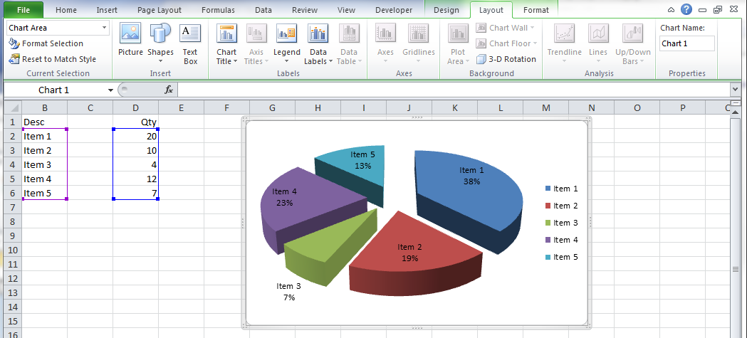
If you want to modify a chart, you can click on the edge of the chart and three new tabs appear on the ribbon (Design, Layout, and Format). In the image above, the Layout tab has been selected and the Data Labels icon was used to display the Category and Percentages for the pie slices.

Select the chart by clicking on its edge. Then right click and choose cut. Click on the worksheet where you want the chart and then right click on that worksheet and click on paste.

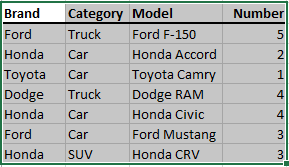
Find the data you want to represent in pivot chart. Make sure the data has descriptive column headings. Select all the data you might want to analyze in your chart and include the headings. Then click on the Insert tab on the ribbon and choose PivotChart.

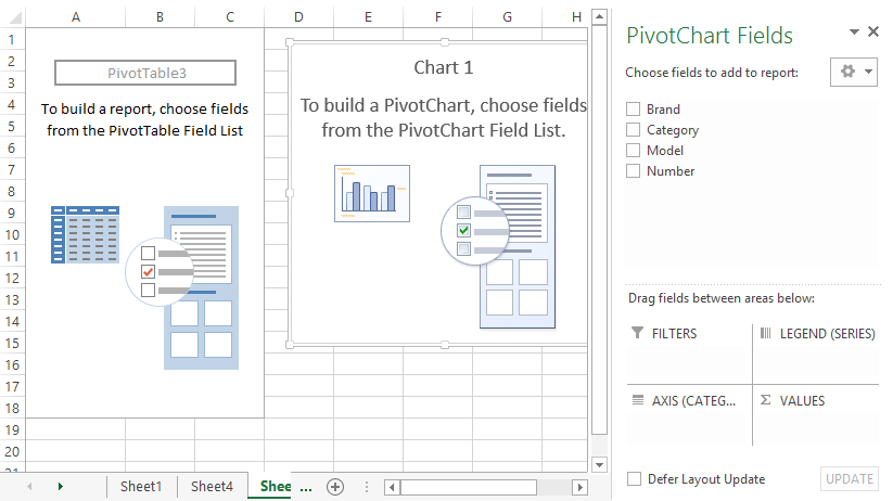
The pivot chart dialog default choices are usually pretty good, so you will usually just want to go with them. Then you should get something that looks like the above. Choose what fields you want to include in the report. In this case, all of them.

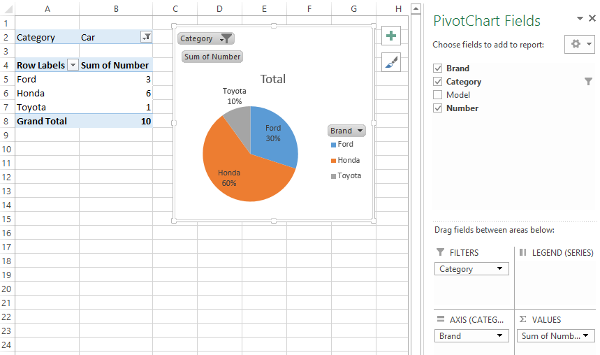
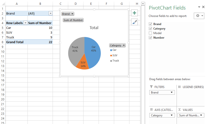
By choosing different options, you can change the chart type, filter the results, and analyze the data quickly in many different ways. In the two examples above, swapping brand and category makes it easy to visualize the percentages for brands, and then for types of vehicles.

The first step in creating a one variable data table in Excel is to set up the basic table with all hard-coded numbers entered. Then enter a correct formula into the first cell of the row or column where the formulas are to go. The following example demonstrates a data table used to calculate the cubes of the integers from 1 through 5.

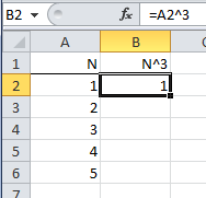
The image above shows the setup just before the data table is created. The headings have been entered. The hard-coded values 1 through 5 have been entered in column A. The first formula has been entered into cell B2. You can see the formula in the formula bar.

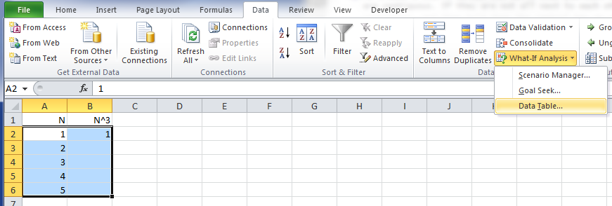
The next step is to select all of the cells in the data table which contain the changing values (A2 through A6 in this case), and the cells where all the formulas will be going (B2 through B6 in this case). The first cell where the formulas will be going must have the formula already filled in (that's B2 in this case). Then click on the ribbon's Data tab and select Data Table from the What-If Analysis drop-down list.

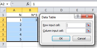
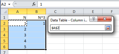
The next step is to tell Excel where the values are that it will be filling in. In this case, the value that will be changing is in cell A2. The new values are in the column below that cell. Therefore you enter A2 into the textbox where it asks for: Column Input Cell. Then click on: OK

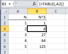
The finished product should look like the table in the image above. Notice how the cryptic formula that Excel creates for you (shown in the formula bar) looks nothing like what we would usually enter as a formula.

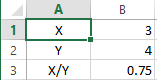
The first step in creating a two variable data table in Excel is to set up some cells with sample values and the basic formula. In this case we are doing a simple division table representing X divided by Y. The example above shows cells for the X and Y values and one for the formula: =B1/B2 (which is X/Y).

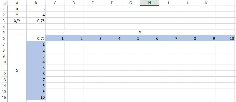
The next step is to create the two dimensional table with changing values for one of the variables in the top row and the other in the leftmost column (non-overlapping). In the example above, those values have been given a blue background color. Then place a reference to the formula to be used in the cell that is the intersection of that row and column. In the example above, cell B6 contains: =B3

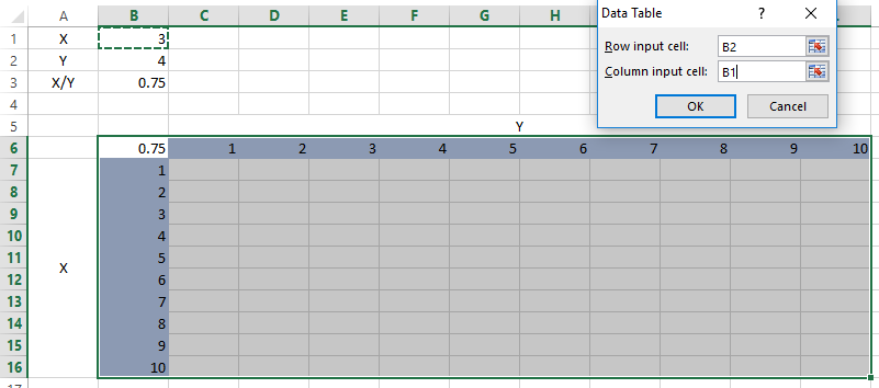
The next step is to create the data table and tell Excel which cell refers to the row values and which refers to the column values. In this case, cell B2 represents Y, which is the row input cell. Cell B1 represents X, which is the column input cell. Click on the ribbon's Data tab and select Data Table from the What-If Analysis drop-down list. Then fill in the correct values for the row and column input cells and click OK.

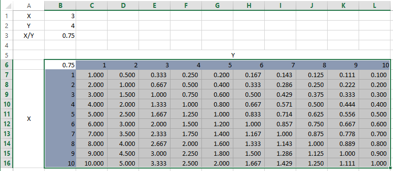
The finished product should look like the table in the image above. You should notice that the cells in the table contain a rather cryptic formula, {=TABLE(B2,B1)}, which looks very different from what we would usually enter as a formula.

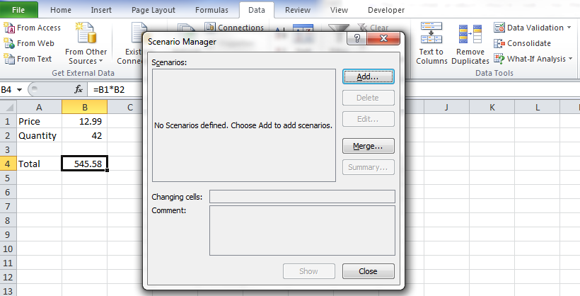
To create a scenario, start on the worksheet that you want the scenarios to summarize. Then click on the ribbon's data tab and choose Scenario Manager from the What-If Analysis drop-down list. Click on Add to create a new Scenario.

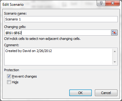
Enter a scenario name and choose which cells will be changing. You will usually want to make sure the Prevent Changes option is checked so your original values remain.

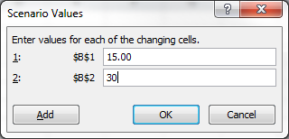
The next step is to enter values for the changing cells.

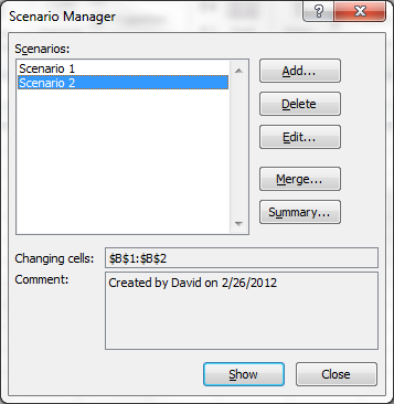
Add as many scenarios as you wish. Then click on the Summary button.

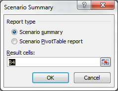
Next you get to choose the type of report that you want and what cell you want see to see what effect your scenarios had on it.

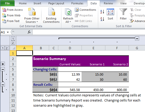
The image above shows the scenario summary report that Excel created.

Start by going to the worksheet that has the data and formulas you want Solver to analyze. Then click on the Solver icon. It is on the Data tab of the ribbon on the far right side. If it isn't there, you will have to install it. The installation instructions are another question on this FAQ. You can go and take care of that now. I'll wait here for you until you get back.

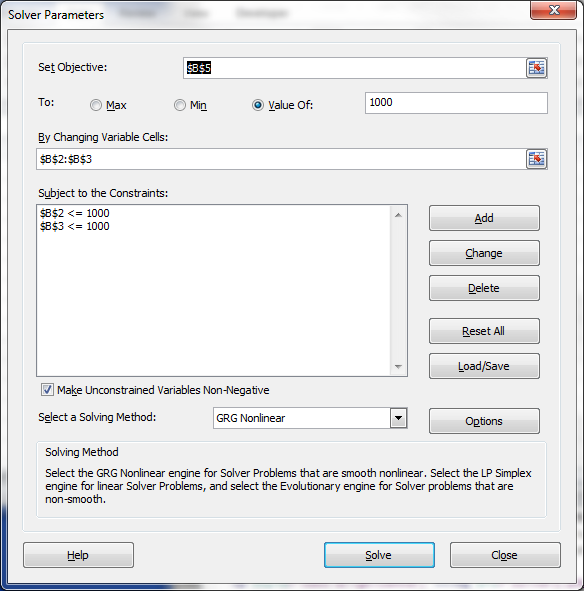
In the Solver dialog, you can set the Objective and which cells Solver is allowed to change to find a solution. You can click on the Add button to add constraints. Click on the Solve button when ready to solve.

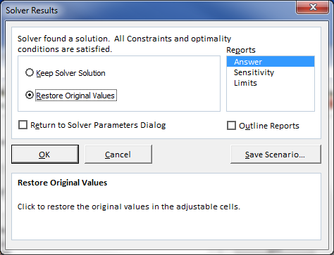
The next step is to choose what type of report you want Excel to generate. In this case we want an Answer report. You will usually want to check the option to restore the original values when Solver is done. Click OK when done.

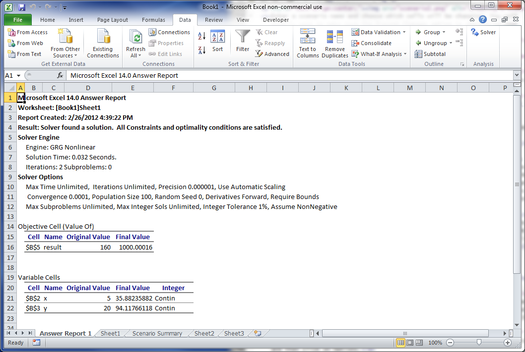
Once you have created a report, it should show up in a new worksheet. Check the worksheet tabs for a new worksheet with a name like: Answer Report 1

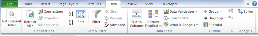
To see if Solver is installed, click on the Data tab of the ribbon and see if Solver shows up at the far right side of the ribbon. If it is there, you have it installed. Otherwise, you will want to install it. The installation steps below are for Excel 2010. Installation for Excel 2007 looks a little different.

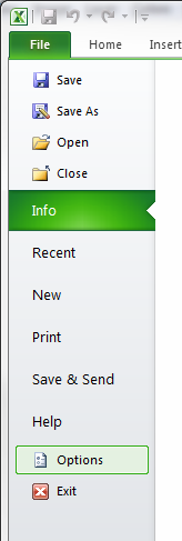
The first step in installing Solver is to click on the File tab of the ribbon and then click on Options.

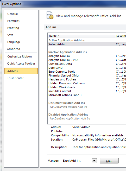
The second step in installing Solver is to click on Add-Ins in the left panel of the Excel Options dialog. Then select Excel Add-ins in the Manage drop-down listbox. Then click on the Go button.

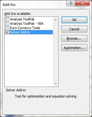
The final step in installing Solver is to check the Solver Add-in and click on OK.

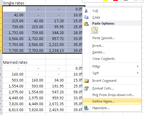
Select the cell(s) you want to define a name for. Then right click on the cell(s) and choose "Define Name...". Enter the name you want for the cells into the dialog box that appears.

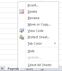
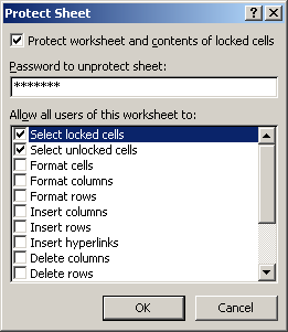
Go to the worksheet you wish to protect. Right click on the worksheet tab at the bottom of the worksheet and choose "Protect Sheet...". Enter a password when requested. You will have to verify the password in a second dialog box.

Protecting individual cells on a worksheet is a multi-step procedure.

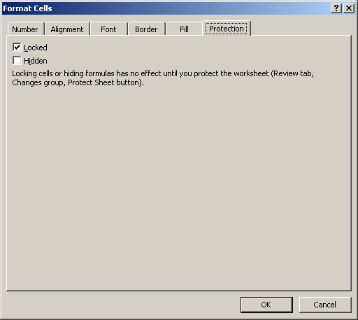
First we must unlock all of the cells on the worksheet. Select all of the cells on the worksheet by clicking on cell A1. Then press Ctrl-A to select all the cells and then right click and choose "Format Cells...". Then click on the "Protection" tab, uncheck the "Locked" checkbox, and click on "OK".

Second, select the cells you want to protect. Then right click on that selection and choose "Format Cells...". Then click on the "Protection" tab, check the "Locked" checkbox, and click on "OK".

Third, protect the worksheet itself. Right click on the worksheet tab at the bottom of the worksheet and choose "Protect Sheet...". Enter a password when requested. You will have to verify the password in a second dialog box.

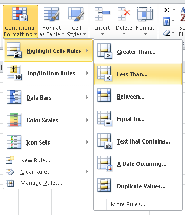
You can modify the format of a cell based on whether it meets specific criteria. Some cases are easy, such as changing the format when a cell is below a certain value. Just select the cell and then click on "Conditional Formatting" on the "Home" tab. Choose "Highlight Cells Rules" on the drop down menu, and then "Less Than...". It should be clear what to do after that. An image of the conditional formatting menu is included below.

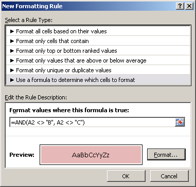
Modifying a cell format based on whether it contains one of two values is more difficult since that is not an option already supplied by Excel. Let us assume we are formatting cell A2 to have a pink background if it is not a B or a C. You start by selecting cell A2. Click on "Conditional Formatting" on the "Home" tab. Then choose "New Rule...", and then choose the "Use a formula to determine which cells to format" option. The formula you would use is an AND function:
=AND(A2 <> "B", A2 <> "C")
What you are literally saying with that formula is that you want to know if the cell does not contain "B" and it does not contain "C".

That's great if you want to apply a format to a cell that is not "B" and is not "C". But what if you want to apply a format to a cell that is equal to either "B" or "C". There is an OR function for that:
=OR(A2 = "B", A2 = "C")

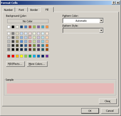
You would click on the "Format..." button to choose what type of formatting you want to give the cell if it meets the criteria you specify.

What if you want to apply multiple conditional formats for a single cell? That is actually quite easy. Just add multiple conditional formats. Excel will use the first one that matches.

So, if you want a blue font when the value is below .25, an orange font when the value is between .25 and .50, and a green font otherwise, just add the three rules. Select the cell. On the Home tab, choose Conditional Formatting, Highlight Cell Rules, Less Than, fill in the value and select the formatting. Then do the same, except the second rule will be for Between, and the third rule will be for Greater Than. Excel will apply the first rule that matches.

The format for using an IF function is: =IF(expression, expression1, expression2)
expression: must evaluate to true or false
expression1: the cell will contain the value of expression1 if expression is true
expression2: the cell will contain the value of expression2 if expression is false

For example, let us assume we are calculating letter grades for a pass/fail class. If the percent grade is greater than or equal to 70% (which is .7 in decimal notation), the letter grade will be "P", otherwise the letter grade will be "F". Let us also assume the percent grade is stored in cell D15. The formula looks like this:
=IF(D15 >= .7, "P", "F")

Please note that the above formula has quotes around some of the values because they are string values. They would not have quotes if they were numbers or expressions to be evaluated. For example, let us assume there is a length in cell A3. If cell B3 is the letter C, then cell A3 represents the radius of a circle. If cell B3 is NOT the letter C, then cell A3 represents the side of a square. We want cell C3 to be the area of that circle or square, so the formula in cell C3 looks like this:
=IF(B3 = "C", 3.14159 * A3 * A3, A3 * A3)
Note: The area of a circle is PI * radius * radius. The area of a square is side * side.

The format of VLOOKUP is: VLOOKUP(value, table, column, rangeLookup)
value: the value you want to translate/lookup in column 1 of the table
table: the defined name (or cell range) of the table we want to use for the lookup
column: the column of the table where the value you want is
rangeLookup: set to true if you want to do a range lookup, otherwise false

Let's assume we are using a table to convert percent grades to letter grades. The table is shown below.

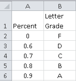
Let us also assume that the grade we want to convert is stored cell E2. If the table has been given a defined name, let's say "Grades", then the formula to use the table to convert the grade is:
=VLOOKUP(E2, Grades, 2, true)
If the table does not have a defined name, you must specify the cell range where the table is located:
=VLOOKUP(E2, $A$2:$B$6, 2, true)